Embrace Multisets: Prime Factorization, GCD, and LCM

Target Audience: Students of mathematics, or computer science in their second semester or higher; or more senior students who want to see applications of multisets. Only surface knowledge of algebra required.

Abstract

This article is the first of a series devoted to highlighting multisets and their occurrences throughout undergraduate mathematics.

For natural numbers, the concepts of prime factorization, divisibility, greatest common divisor ($\gcd$), and least common multiple ($\mathrm{lcm}$) are widespread in many branches of mathematics. Students learn about them in their first semesters; if not even earlier at school. However, usually lesser known are the multiset-theoretic interpretations of these concepts. Here, we define a variant of multisets from the ground up, and show the usefulness of identifying natural number with their multiset of prime factors. That way, multiplication and division become multiset union and difference, respectively, and $\gcd$ and $\mathrm{lcm}$ become multiset intersection and symmetric difference.

We focus on expressing these correspondences algebraically. We recap the theory of lattices and obtain a lattice-isomorphism $L_{\mathbb{N}}\cong M_{{\mathbb{P}}^{+}}$ between the division lattice on natural numbers and the lattice of finite multisets over prime numbers with multiplicities in ${\mathbb{N}}_{\ge 0}$. By generalizing the right-hand side to the superlattice $M_{\mathbb{P}}$, now with multiplicities in ℤ, we recover a useful generalization of the left-hand side: a division lattice on $\mathbb{Q}⁺$. In particular, we prove multiset intersection and symmetric difference on $M_{\mathbb{P}}$ to correspond on $\mathbb{Q}⁺$ to generalized variants of $\gcd$ and $\mathrm{lcm}$ fulfilling $$\begin{array}{rl}\gcd (\frac{a}{b},\frac{c}{d})& =\frac{\gcd (a,c)}{\mathrm{lcm}(b,d)}\\ \mathrm{lcm}(\frac{a}{b},\frac{c}{d})& =\frac{\mathrm{lcm}(a,c)}{\gcd (b,d)}\end{array}$$ for reduced fraction representations $\frac{a}{b}$ and $\frac{c}{d}$.

1 Introduction

The central idea is the following. Every natural number $n\ge 2$ can be factored into its prime factors. Since multiplicity of prime factors is crucial, but order is not, the prime factorization of a natural number forms a multiset. For example, we have $18=2\cdot 3^2$ and can thus identify $18$ with the multiset $\{2^{(1)},3^{(2)}\}$, where the exponents denote multiplicities, i.e., $2$ occurs once and $3$ occurs twice. By extending the identification to $n=1$ with the empty multiset, we obtain the bijections below between the natural numbers $\mathbb{N}=\{1,2,\dots \}$ and the set $M_{{\mathbb{P}}^{+}}$ of finite multisets with multiplicities in ${\mathbb{N}}_{\ge 0}$. $$\begin{array}{rl}\mathrm{fact}& :\mathbb{N}\to M_{{\mathbb{P}}^{+}}\\ \mathrm{mult}& :M_{{\mathbb{P}}^{+}}\to \mathbb{N}\end{array}$$ Here, $\mathrm{fact}$ maps every natural number to its prime factorization, and $\mathrm{mult}$ maps every multiset of primes to a natural number by multiplying, counting multplicities.

This article is driven by the following questions: Can we say more than $\mathbb{N}\cong M_{{\mathbb{P}}^{+}}$ as sets? That is, is this an isomorphism of more than just sets? For example, how do common operations on natural numbers like multiplication, division, greatest common divisor ($\gcd$), and least common multiple ($\mathrm{lcm}$) look like on the side of $M_{{\mathbb{P}}^{+}}$? Does $\mathrm{fact}$ preserve and reflect them?

Indeed, we will see that $\gcd$, $\mathrm{lcm}$ of natural numbers correspond to multiset intersection and symmetric difference; both counting multiplicities in a suitable manner. Algebraically, these operation pairs make each side of $\mathbb{N}\cong M_{{\mathbb{P}}^{+}}$ into a lattice. On the left-hand side, we have the division lattice $(\mathbb{N},\gcd ,\mathrm{lcm})$, and on the right-hand side, we obtain the lattice $(M_{{\mathbb{P}}^{+}},\cap ,\Delta )$ of finite multisets with non-negative multiplicities equipped with multiset intersection and symmetric difference. In our main theorem, we prove that the properties of $\mathrm{fact}$ and $\mathrm{mult}$ extend accordingly, i.e., the functions defined above are in fact lattice isomorphisms.

Overview. We rigorously define multisets and their operations in Section 2.1. In Section 2.2 we recap the theory of lattices and detail the lattices involved above. Then, in Section 3 we prove our main theorem showing $\mathbb{N}\cong M_{{\mathbb{P}}^{+}}$ as lattices. In Section 4, we extend the lattices on both sides and obtain a generalized theorem. We conclude in Section 5.

2 Preliminaries

We work in the usual metamathematical layer and remain vague about our foundation. We, however, do presuppose some kind of set theory, e.g. ZF. To avoid confusion with multisets later, let us refer to sets from the designated set theory as classical sets, and to multisets always as multisets.

2.1 Multisets

2.1.1 Definitions

Classical sets are “collections of objects” without order and without duplicates. That is, an object is either element of a classical or is it not. Multisets, which have been folklore for long time, lift the latter requirement and instead attach to every element a multiplicity. For our purposes, we define multiplicities to be integers. Other domains may call for different choices, e.g. fuzzy sets, where elementhood is interpreted probabilistically, can be seen as multisets with multiplicities in $[0,1]\subseteq ℝ$.

Definition 2.1 [¹]: A multiset is a pair $(U,{\kappa }_U)$, where $U$ is a classical set and ${\kappa }_U:U\to \mathbb{Z}$ a function.

For $x\in U$, we say $x$ has multiplicity ${\kappa }_U(x)$, or equivalently, $x$ occurs ${\kappa }_U(x)$ times in $(U,{\kappa }_U)$.

If it is clear from context, we write $U$ instead of $(U,{\kappa }_U)$.

Every classical set $S$ can be identified with the multiset $(S,s\mapsto 1)$. For instance, consider the multiset on $U=\{a,b,c\}$ in which $a$ occurs once, $b$ twice, and $c$ -4 times. Formally, we have ${\kappa }_U=\{a\mapsto 1,b\mapsto 2,c\mapsto -4\}$. In the following we adopt an easier notation for concrete multisets and write $\{a^{(1)},b^{(2)},c^{(-4)}\}$.

We would like to treat two multisets as equal even if their associated functions do not have a common domain, e.g. it should hold $\{a^{(1)}\}=\{a^{(1)},b^{(0)}\}$. Therefore, we identify multisets $U_1$ and $U_2$ if ${\kappa }_1$ and ${\kappa }_2$ agree on all urelements of our set theory where at least one of them is non-zero. This allows us to speak of the empty multiset, which we denote by $\varnothing$.

Definition 2.2: Given two multisets $U_1,U_2$, we define

• the union $$U_1\cup U_2:=(U_1\cup U_2,x\mapsto {\kappa }_1(x)+{\kappa }_2(x))$$
• the intersection $$U_1\cap U_2:=(U_1\cup U_2,x\mapsto min\{{\kappa }_1(x),{\kappa }_2(x)\})$$
• the symmetric difference $$U_1\Delta U_2:=(U_1\cup U_2,x\mapsto max\{{\kappa }_1(x),{\kappa }_2(x)\})$$
• the negative $$-U_1:=(U_1,x\mapsto -{\kappa }_1(x))$$
• the difference $$U_1-U_2:=(U_1\cup U_2,x\mapsto {\kappa }_1(x)-{\kappa }_2(x))$$

where we take ${\kappa }_1(x)$ and ${\kappa }_2(x)$ to be $0$ if $x$ lies outside their domain, respectively.

For example, we have:

• $\{a^{(2)},b^{(4)}\}\cup \{a^{(-5)}\}=\{a^{(-3)},b^{(4)}\}$
• $\{a^{(2)},b^{(3)}\}\cap \{a^{(10)},b^{(-5)}\}=\{a^{(2)},b^{(-5)}\}$
• $\{a^{(2)},b^{(3)}\}\Delta \{a^{(10)}\}=\{a^{(10)},b^{(3)}\}$

Definition 2.3: We say $U$ is finite if ${\kappa }_U(x)\ne 0$ only for finitely many $x$.

In the sequel, we will be working with multisets that may only contain prime numbers. In general, almost always we only work with multisets over a designated classical set, as defined below.

Definition 2.4 (Multisets over a Classical Set): Let $X$ be a classical set. Then, define

• $M_X$ to be the classical set of all finite multisets with elements only in $X$.
• $M_{X^{+}}$ to be subset of $M_X$ where we only allow non-negative multiplicities.

2.1.2 Prime Factorization as a Multiset

For the rest of this article, let $\mathbb{N}=\{1,2,\dots \}$ denote the natural numbers without zero and $\mathbb{P}=\{2,3,5,\dots \}$ the prime numbers. Prime factorization allows us to factor every natural number $n\ge 2$ into its prime factors, which form a multiset. For example, we can identify $18=2\cdot 3^2$ with the multiset $\{2^{(1)},3^{(2)}\}$.

Overall, this gives rise to the bijections $$\begin{array}{rl}\mathrm{fact}& :\mathbb{N}\to M_{{\mathbb{P}}^{+}}\\ \mathrm{mult}& :M_{{\mathbb{P}}^{+}}\to \mathbb{N}\end{array}$$ where $\mathrm{fact}$ maps every natural number to its prime factorization, and $\mathrm{mult}$ maps every multiset of primes to a natural number by multiplying, counting multplicities. By convention, we set $\mathrm{fact}(1)=\varnothing$ and $\mathrm{mult}(\varnothing )=1$.

We have the following exemplary correspondences:

These correspondences hold in general: $\mathrm{fact}$ is a homomorphism wrt. the operations multiplication, $\gcd$, and $\mathrm{lcm}$, and translates these operations into multiset union, intersection, and symmetric difference. Analogously for $\mathrm{mult}$, which preserves unions, intersections, and symmetric differences, and translates everything into the other direction. The list below formally summarizes these properties, quantified over all $a,b\in \mathbb{N}$ and $A,B\in M_{{\mathbb{P}}^{+}}$. We defer proving these identities until Section 3, at which point we will have introduced enough multiset and algebra machinery to allow for a concise proof.

$$\begin{array}{rl}\mathrm{fact}(a\cdot b)& =\mathrm{fact}(a)\cup \mathrm{fact}(b)\\ \mathrm{fact}(\gcd (a,b))& =\mathrm{fact}(a)\cap \mathrm{fact}(b)\\ \mathrm{fact}(\mathrm{lcm}(a,b))& =\mathrm{fact}(a)\Delta \mathrm{fact}(b)\\ \mathrm{mult}(A\cup B)& =\mathrm{mult}(A)\cdot \mathrm{mult}(B)\\ \mathrm{mult}(A\cap B)& =\gcd (\mathrm{mult}(A),\mathrm{mult}(B))\\ \mathrm{mult}(A\Delta B)& =\mathrm{lcm}(\mathrm{mult}(A),\mathrm{mult}(B))\end{array}$$

Remark 2.5: The division ${\frac{a}{b}}_{\mathbb{N}}$ of two natural numbers over ℕ corresponds to multiset difference only if its result is a natural number again. For example,

$$\mathrm{fact}\left(\frac{14}{2}\right)=\mathrm{fact}(14)-\mathrm{fact}(2)$$

but, depending on your definition, ${\frac{14}{6}}_{\mathbb{N}}=2$, whereas $\mathrm{fact}(14)-\mathrm{fact}(6)$ corresponds to not a single natural number as it contains elements with negative multiplicities.

2.1.3 Technical Lemmas

In the following, we collect some technical lemmas concerning multisets. Of central interest for the proofs of our main theorems will be Lemmas 2.7 — 2.9.

Lemma 2.6:

1. Union, intersection, symmetric difference are commutative and associative operations.
2. The negative is an involution.
3. $U_1-U_2=U_1\cup (-U_2)$
4. $U_1\cap U_2=(U_1\cup U_2)-(U_1\Delta U_2)=-(-U_1\Delta -U_2)$
5. $U_1\Delta U_2=(U_1\cup U_2)-(U_1\cap U_2)=-(-U_1\cap -U_2)$

Lemma 2.7: Intersection and symmetric difference are related as follows:

1. $U_1\cap (U_2\Delta U_3)=(U_1\cap U_2)\Delta (U_1\cap U_3)$
2. $U_1\Delta (U_2\cap U_3)=(U_1\Delta U_2)\cap (U_1\Delta U_3)$

The theory of multisets also admits the decomposition theorem below, splitting a multiset into elements of positive and of negative multiplicity. We note that this theorem comes at no surprise given that we proved the negative to be an involution — since generally in mathematics, involutions often go hand-in-hand with decomposition theorems.

Lemma 2.8 (Sign Decomposition): Let $U$ be a multiset, then $U=U⁺-U⁻$ with

• positive part $U⁺:=\{x\in U\mid {\kappa }_U(x)>0\}=U\Delta \varnothing$ and
• negative part $U⁻:=\{x\in U\mid {\kappa }_U(x)<0\}=U\cap \varnothing$

We can express intersection and symmetric difference using sign decompositions as follows.

Lemma 2.9: Let $U$ and $V$ be multisets, then

• $$U\cap V=(U⁺\cap V⁺)-(U⁻\Delta V⁻)$$
• $$U\Delta V=(U⁺\Delta V⁺)-(U⁻\cap V⁻)$$

The proofs of the latter two lemmas are left to the reader. Note that the second point of Lemma 2.9 follows by duality from the first point.

2.2 Lattices

Recall we equipped the natural numbers with $\gcd$ and $\mathrm{lcm}$ to arrive at the triple $(\mathbb{N},\gcd ,\mathrm{lcm})$; and the multisets over primes $M_{{\mathbb{P}}^{+}}$ with intersection and symmetric difference to arrive at $(M_{{\mathbb{P}}^{+}},\cap ,\Delta )$. Moreover, we had functions $\mathrm{fact}$ and $\mathrm{mult}$ bijecting the underlying sets. In this section, our goal is to see these things from an algebraic perspective. Concretely, we motivate the theory of lattices: a suitable theory that makes these triples into lattices and the bijections into lattice isomorphisms.

Let us begin with some motivation. Roughly, we can think of (mathematical) lattices as modeling real-world lattices such as the one in Figure 1.

Intuitively, a real-world lattice has two characteristics: its collection of nodal points and its mesh structure. How we encode this in mathematics? Straightforwardly, we encode the former as a classical set $L$, e.g., for the lattice in Figure 1 we have $L=\mathbb{N}₀\times \mathbb{N}₀$. Representing the mesh structure requires more care since naively choosing graphs on $L$ for it would disregard the additional structure real-world (and mathematical lattices) often have. For example, any two nodal points have common ancestors and descendants, and moreover there is a unique ancestor (descendant) that is nearest, in some distance sense, to two given nodal points. These things do not hold in arbitrary graphs; hence graphs are too generous to model lattices. Instead, we model lattices by two functions $\vee ,\wedge :L\times L\to L$ called meet and join, of which we think as picking those unique ancestors and descendants for any two nodal points.

Let us better understand those unique points and operations by means of the lattice in Figure 1. Imagine you are standing on $(0,1)$ and your friend on $(5,0)$. You would like to gather at some common point, but both of you can only walk downwards for some reason. Which point can you gather at such that both of you only travel the minimum distance necessary? At $(5,0)$, and even uniquely so. This is the “unique ancestor” we referred to above. We encode this using the meet operation as $(0,1)\vee (5,0)=(5,0)$. Now on the contrary, imagine you both could only walk upwards starting from $(0,1)$ and $(5,0)$, respectively. We again ask the question: Which point can you gather at such that both of you only travel the minimum distance necessary? At $(5,1)$, again uniquely so. We encode this “unique descendant” as the join $(0,1)\wedge (5,0)=(5,1)$. Can you derive general formulae for meets and joins for the lattice on $L=\mathbb{N}₀\times \mathbb{N}₀$ represented in Figure 1?

With the imaginery above, it is also clear meet and join ought to be commutative and associative operations. Here, associativity says that when three people $p_1,p_2,p_3$ would like to gather, e.g., by only walking upwards, then there is a unique gathering point independent of whether they gather up “in parallel” ($p_1\wedge p_2\wedge p_3$), by the first two people gathering first ($(p_1\wedge p_2)\wedge p_3$), or by the latter two people gathering first ($p_1\wedge (p_2\wedge p_3)$).

Definition 2.10: A lattice is a structure $(L,\vee ,\wedge )$ consisting of a classical set $L$ and two commutative and associative operations $\vee ,\wedge :L\times L\to L$ fulfilling the absorption laws $$\begin{array}{rl}a\vee (a\wedge b)& =a\\ a\wedge (a\vee b)& =a\end{array}$$

We leave it to the reader to motivate and prove the absorption laws in context of Figure 1. Thus, $(\mathbb{N}₀\times \mathbb{N}₀,min,max)$ is a lattice.

Remark 2.11: Lattices can be equivalently described from an order-theoretical perspective: lattices are partially ordered classical sets where each the classical set possseses a greatest lower bound (also: meet) and least upper bound (join) for every two-element subset $\{a,b\}$. We refer to Wikipedia for a definition of these bounds.

It often helps to think of lattices in terms of both the algebraic and order-theoretical perspective. The example lattice from above corresponds to $\mathbb{N}₀\times \mathbb{N}₀$ partially ordered by $$(a,b)⊑(c,d)\iff (a⊑c)\text{ and }(b⊑d).$$ In particular, lattices are usually drawn as Hasse diagrams, as was done in Figure 1: every upwards edge $x–y$ stands for $x⊑y$.

Remark 2.12: Lattice in which additionally meet and join distribute over each other, as below, are called distributive lattices. $$\begin{array}{rl}a\vee (b\wedge c)& =(a\vee b)\wedge (a\vee c)\\ a\wedge (b\vee c)& =(a\wedge b)\vee (a\wedge c)\end{array}$$

2.2.1 Divison Lattice on ℕ

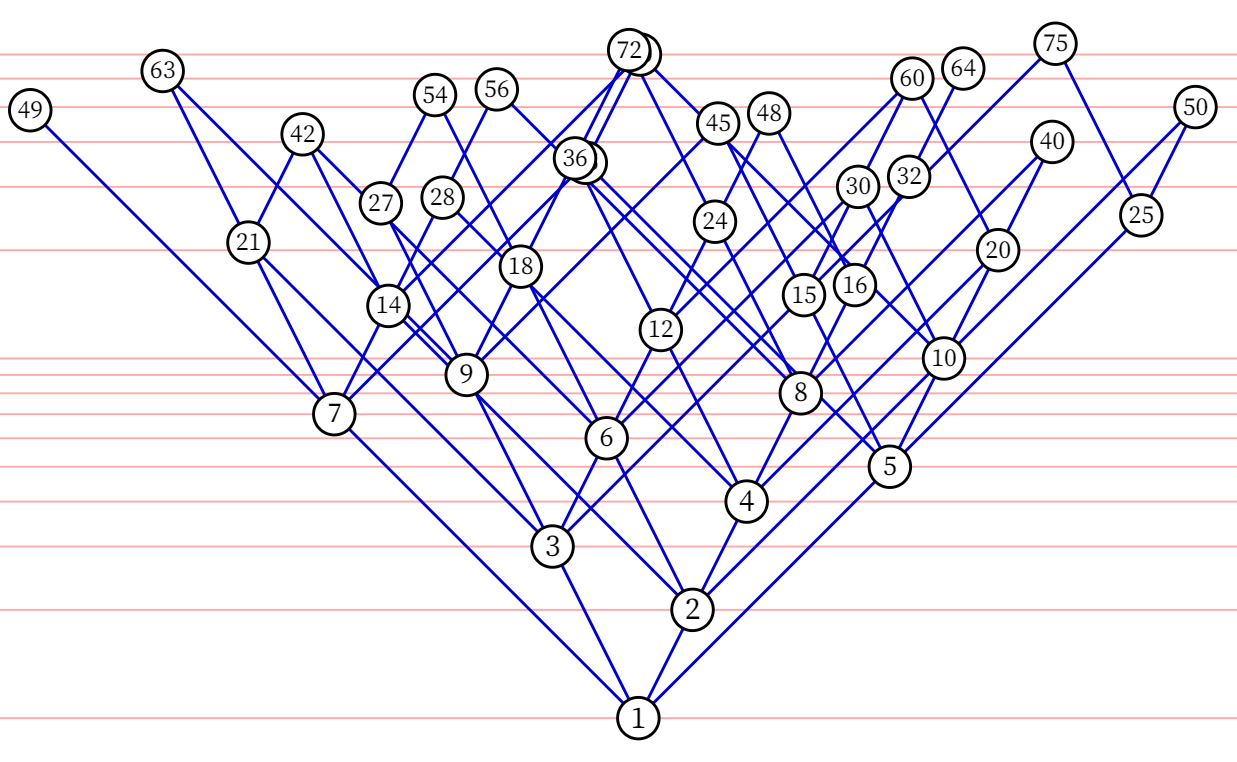
Given two natural numbers $n$ and $m$, we define the well-known divisibility relation $$n\mid m\iff \exists q\in \mathbb{N}.n\cdot q=m$$ This is a partial order, and moreover for every two-element subset, the greatest common divisor and the least common multiple serve as meets and joins, respectively.

Lemma 2.13 (Division Lattice on ℕ): $L_{\mathbb{N}}:=(\mathbb{N},\gcd ,\mathrm{lcm})$ is a lattice.

See Figure 2 for a partial visualization of $L_{\mathbb{N}}$ as a Hasse diagram. For example, the meet of 18 and 12 is $6=\mathrm{lcm}(18,12)$, and 6 is precisely the nearest point you can reach from both 18 and 12 by only walking downards. Also, the join of 2 and 5 is $10=\gcd (2,5)$, and 10 is precisely the nearest point you can reach from both 2 and 5 by only walking the edges upwards.

Remark 2.14: In the division lattice on ℕ, the element 1 has the property that it divides every other number, i.e., order-theoretically $1⊑n$ for all $n$. Lattices that possess such a bottom element are called lower-bounded lattices.

2.2.2 Multiset Lattices

Let $X$ be a classical set. Then we can put a lattice structure on the multisets over $X$ by ordering them by $$U_1⊑U_2\iff \forall x\in U_1.{\kappa }_1(x)\le {\kappa }_2(x).$$ See Figure 3 for a partial visualization of the corresponding Hasse diagram. From an algebraic point of view, the meet and join of two multisets are precisely the intersection and symmetric difference, respectively. For example, we have the joins

• $\{a^{(1)}\}\Delta \{b^{(2)}\}=\{a^{(1)},b^{(2)}\}$
• $\{a^{(1)},b^{(1)}\}\Delta \{b^{(2)}\}=\{a^{(1)},b^{(2)}\}$

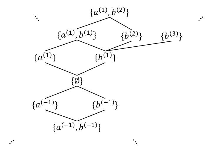
Theorem 2.15 (Multiset Lattices): Let $X$ be a classical set.

1. $(M_X,\cap ,\Delta )$ is a distributive lattice.

2. $(M_{X^{+}},\cap ,\Delta )\subseteq M_X$ is a distributive sublattice with bottom $\varnothing$

We leave the proof to the reader.

Remark 2.16: On first sight, the reader might wonder why the join operation for the multiset lattice is symmetric difference and not union. After all, in contrast, with classical sets all subsets of $X$ form a lattice wrt. classical intersection and classical union. This lattice is known as the powerset lattice.

When generalizing to multisets, however, the classical union must not become multiset, but instead symmetric difference. This can be seen in the example from above: the join of $\{a^{(1)},b^{(1)}\}$ and $\{b^{(2)}\}$ is $\{a^{(1)},b^{(2)}\}$. It is clear that the latter is the order-theoretical join (wrt. $⊑$ given above). A multiset union of both operands would result in $\{a^{(1)},b^3\}$, counting $b$ three times. The symmetric difference avoids such overcounting.

Remark 2.17: Ignoring size issues of the chosen set theory, the class of all multisets would form a lattice, too.

3 Divison Lattice on ℕ ≅ Positive Finite Multisets over ℙ

With the preliminaries done, we can finally state and prove our main theorem: the division lattice on ℕ can be identified with the lattice of positive finite multisets over primes.

Theorem 3.1: $L_{\mathbb{N}}\cong M_{{\mathbb{P}}^{+}}$ as lower-bounded lattices, where

• $\mathrm{fact}:L_{\mathbb{N}}\to M_{{\mathbb{P}}^{+}}$ maps natural numbers to their prime factorization
• $\mathrm{mult}:M_{{\mathbb{P}}^{+}}\to L_{\mathbb{N}}$ maps multisets of primes to their multiplication

Moreover, multiplication is preserved and reflected as multiset union:

$$\begin{array}{rl}\mathrm{fact}(a\cdot b)& =\mathrm{fact}(a)\cup \mathrm{fact}(b)\\ \mathrm{mult}(A\cup B)& =\mathrm{mult}(A)\cdot \mathrm{mult}(B)\end{array}$$

4 Division lattice on ℚ⁺ ≅ Finite Multisets over ℙ

We have seen $L_{\mathbb{N}}\cong M_{{\mathbb{P}}^{+}}$, i.e., how the division lattice on ℕ is isomorphic to the lattice of positive finite multisets over primes. What happens if we now relax (extend) the RHS to the superlattice $M_{\mathbb{P}}$ with negative multiplicities allowed, too? Is there also a corresponding superlattice of $L_{\mathbb{N}}$ that is isomorphic to $M_{\mathbb{P}}$? Indeed there is, and a natural generalization of $L_{\mathbb{N}}$ to a division lattice $L_{\mathbb{Q}⁺}$ on ℚ⁺ fits the bill, where $\mathbb{Q}⁺=\{q\in \mathbb{Q}\mid q>0\}$ are the positive rational numbers. In particular, this yields meaningful extensions of $\gcd$ and $\mathrm{lcm}$ to ℚ⁺.

Before defining $L_{\mathbb{Q}⁺}$ and proving $L_{\mathbb{Q}⁺}\cong M_{\mathbb{P}}$, let us begin with building some intuition as to why that should be the case. Recall how we bijected positive finite multisets over ℙ with natural numbers: we mapped a multiset $A$ to the multiplication ${\mathrm{\Pi }}_{p\in \mathbb{P}}{p}^{{\kappa }_A(p)}$. What happens if we allowed negative multiplicities, i.e., ${\kappa }_A(p)<0$? Nothing, really; multiplying prime factors raised to possibly negative exponents still makes sense. For example, we would map $\{5^{(1)},2^{(-1)},3^{(-2)}\}$ to $5^1\cdot 2^{-1}\cdot 3^{-2}=\frac{5}{18}$. Hence, we represent fractions as multisets with prime factors of their numerator becoming positive elements and prime factors of their denominator becoming negative elements. To ensure uniqueness, we always choose the reduced fraction representation.

Definition 4.1 (Prime Factorization of Rational Numbers): Let $r\in \mathbb{Q}⁺$ be a rational number with reduced fraction representation $\frac{a}{b}$ with $a,b\in \mathbb{N}$. Let $a=p_1^{a_1}\cdot \dots \cdot p_n^{a_n}$ and $b=q_1^{b_1}\cdot \dots \cdot q_m^{b_m}$ be the prime factorizations of $a$ and $b$ with $n,m\ge 0$. Then, we call $$r=p_1^{a_1}\cdot \dots \cdot p_n^{a_n}\cdot q_1^{-b_1}\cdot \dots \cdot q_m^{-b_m}.$$ the prime factorization of $r$.

By convention, we set $1=⟨\text{empty product}⟩$.

This allows identifying rational numbers with multisets of their prime factors. In contrast to earlier discussions, we must now allow multiplicities in ℤ.

Definition 4.2 (Lattice on ℚ⁺): Define the lattice $L_{\mathbb{Q}⁺}=(\mathbb{Q}⁺,\gcd ,\mathrm{lcm})$ with

• $$\gcd (\frac{a}{b},\frac{c}{d})=\frac{\gcd (a,c)}{\mathrm{lcm}(b,d)}$$
• $$\mathrm{lcm}(\frac{a}{b},\frac{c}{d})=\frac{\mathrm{lcm}(a,c)}{\gcd (b,d)}$$

Here, we overload the names of $\gcd$ and $\mathrm{lcm}$ as the functions defined here agree with the previously defined functions when restricted to ℕ. We leave proving the lattice properties to the reader.

For example, we have $\gcd (\mathrm{⅜},\mathrm{⅖})=\frac{\gcd (3,2)}{\mathrm{lcm}(8,5)}=\frac{1}{40}$. Moreover, $\mathrm{lcm}(\mathrm{⅜},\mathrm{⅖})=\frac{\mathrm{lcm}(3,2)}{\gcd (8,5)}=\frac{6}{1}$, and indeed, $6$ is the first common multiple of both $\mathrm{⅜}$ and $\mathrm{⅖}$.

Theorem 4.3: $L_{\mathbb{Q}⁺}\cong M_X$ as lattices, where

• $\mathrm{fact}:L_{\mathbb{Q}⁺}\to M_{\mathbb{P}}$ maps rational numbers to their prime factorization
• $\mathrm{mult}:M_{\mathbb{P}}\to L_{\mathbb{Q}⁺}$ maps multisets of primes to their multiplication

Moreover, multiplication and division are preserved and reflected as follows: $$\begin{array}{rl}\mathrm{fact}(a\cdot b)& =\mathrm{fact}(a)\cup \mathrm{fact}(b)\\ \mathrm{fact}\left(\frac{a}{b}\right)& =\mathrm{fact}(a)-\mathrm{fact}(b)\\ \mathrm{mult}(A\cup B)& =\mathrm{mult}(A)\cdot \mathrm{mult}(B)\\ \mathrm{mult}(A-B)& =\frac{\mathrm{mult}(A)}{\mathrm{mult}(B)}\end{array}$$

Again, we overload the names of $\mathrm{mult}$ and $\mathrm{fact}$.

5 Future Work

Both of our main theorems 3.1 and 4.3 state a lattice isomorphism to capture the correspondence between $\gcd$, $\mathrm{lcm}$ and multiset intersection and symmetric difference. Moreover, both theorems guarantee that the respective lattice isomorphism preserves more structure. In case of Theorem 3.1, the lattice isomorphism also preserves multiplication on natural numbers as multiset union. And in case of Theorem 4.3, the isomorphism additionally preserves division on rational numbers as multiset difference. Algebraically, what do these additional preservation properties mean? Is there a known concept in algebra subsuming lattices that would allow us to concisely express them?

We will answer this affirmatively in a future post, namely with lattice-ordered monoids and lattice-ordered groups.

TODO for Author

• Delta has wrong spacing because it’s not a binary operator for tex
• Answer here: https://math.stackexchange.com/questions/151081/gcd-of-rationals